Tucson Crime Analysis
Abstract
This post will cover in some detail a project taken on by myself and two peers. To see a more detailed and academic presentation of our findings please see:
Overview
This project analyzes how reported crime patterns in Tucson relate to (1) neighborhood income and (2) the presence of streetlights. I focused on two main hypotheses:
- Crime vs. Wealth: do thefts and violent crimes occur more often in richer or poorer areas?
- Crime vs. Streetlights: does streetlight presence influence crime rates, especially at night?
The pipeline combines data cleaning + feature engineering, exploratory visualization, and several models (Ridge Regression, Random Forest, Logistic Regression, and OLS).
Data sources (inputs)
- Tucson Police Reported Crimes (CSV)
- Tucson Police Arrests (CSV)
- City of Tucson Streetlight Locations (CSV)
- Neighborhood Income (CSV)
Loading + preprocessing
A key step was normalizing time fields (extracting an hour from TimeOccur) and building a time period label to support night-crime analysis.
# Convert DateOccurred to datetime
crime_df["DateOccurred"] = pd.to_datetime(crime_df["DateOccurred"], errors="coerce")

def extract_hour(time_str):
    try:
        time_str = str(time_str).strip()
        if time_str.isdigit() and 3 <= len(time_str) <= 4:
            time_str = time_str.zfill(4)
            hour = int(time_str[:2])
            if 0 <= hour <= 23:
                return hour
        return np.nan
    except (ValueError, TypeError):
        return np.nan

crime_df["Hour"] = crime_df["TimeOccur"].apply(extract_hour)

def categorize_time(hour):
    if pd.isna(hour): return "Unknown"
    elif 5 <= hour < 12: return "Morning"
    elif 12 <= hour < 17: return "Afternoon"
    elif 17 <= hour < 22: return "Evening"
    else: return "Night"

crime_df["Time_Period"] = crime_df["Hour"].apply(categorize_time)

# Filter years and remove rows missing critical fields
crime_df = crime_df[crime_df["Year"].isin([2018, 2019, 2020, 2021, 2022, 2023, 2024, 2025])]
crime_df = crime_df.dropna(subset=["Ward", "UCRDescription", "DateOccurred", "Hour"])
crime_df.loc[:, "Ward"] = crime_df["Ward"].astype(int)
Building ward-level features + integrating datasets
To comprare areas consistently, we aggregated everything by ward:
Crime_Count: total reported crimes per wardArrest_Count: total arrests perwardNight_Crime_Prop: proportion of crimes occurring at nightStreetlight_Count: streetlights assigned to by wards via nearest spatial join using GeoPandas
# Aggregate crime and arrest counts by ward
crime_by_ward = crime_df.groupby("Ward", observed=False).size().reset_index(name="Crime_Count")
arrest_by_ward = arrest_df.groupby("WARD", observed=False).size().reset_index(name="Arrest_Count")

# Proportion of nighttime crimes per ward
night_crimes = (
    crime_df[crime_df["Time_Period"] == "Night"]
    .groupby("Ward", observed=False).size()
    .reset_index(name="Night_Crime_Count")
)
total_crimes = crime_df.groupby("Ward", observed=False).size().reset_index(name="Total_Crime_Count")
night_crime_prop = night_crimes.merge(total_crimes, on="Ward")
night_crime_prop["Night_Crime_Prop"] = night_crime_prop["Night_Crime_Count"] / night_crime_prop["Total_Crime_Count"]
night_crime_prop = night_crime_prop[["Ward", "Night_Crime_Prop"]]

# Merge with income data (ward key)
merged_df = income_df.merge(crime_by_ward, left_on="WARD", right_on="Ward", how="left")
merged_df = merged_df.merge(arrest_by_ward, on="WARD", how="left")
merged_df = merged_df.merge(night_crime_prop, left_on="WARD", right_on="Ward", how="left")
merged_df = merged_df.drop(columns=["Ward"], errors="ignore")

# Spatial join: assign streetlights to wards using nearest arrest geometry
arrest_gdf = gpd.GeoDataFrame(
    arrest_df,
    geometry=[Point(xy) for xy in zip(arrest_df["X"], arrest_df["Y"])],
    crs="EPSG:2868",
)
streetlight_gdf = gpd.GeoDataFrame(
    streetlight_df,
    geometry=[Point(xy) for xy in zip(streetlight_df["X"], streetlight_df["Y"])],
    crs="EPSG:2868",
)

streetlight_by_ward = gpd.sjoin_nearest(
    streetlight_gdf,
    arrest_gdf[["WARD", "geometry"]],
    how="left",
    max_distance=1000,
)
streetlight_count = streetlight_by_ward.groupby("WARD").size().reset_index(name="Streetlight_Count")

merged_df = merged_df.merge(streetlight_count, on="WARD", how="left")
merged_df["Streetlight_Count"] = merged_df["Streetlight_Count"].fillna(0)
Exploratory Analysis
We used a correlation heatmap and a scatter plot to sanity-check relationships between:
- income (
MEDHINC_CY,AVGHINC_CY) - ward crime and arrests
- streetlight counts
- night-crime proportion
correlation_matrix = merged_df[
    ["MEDHINC_CY", "AVGHINC_CY", "Streetlight_Count", "Crime_Count", "Arrest_Count", "Night_Crime_Prop"]
].corr()

plt.figure(figsize=(10, 8))
sns.heatmap(correlation_matrix, annot=True, cmap="coolwarm", center=0)
plt.title("Correlation Matrix of Income, Streetlights, Night Crimes, and Crime/Arrests")
plt.show()

plt.figure(figsize=(12, 8))
sns.scatterplot(
    data=merged_df,
    x="MEDHINC_CY",
    y="Crime_Count",
    size="Streetlight_Count",
    hue="Night_Crime_Prop",
)
plt.title("Crime Count vs Median Household Income (size=streetlights, hue=night crime)")
plt.xlabel("Median Household Income ($)")
plt.ylabel("Crime Count")
plt.show()
Modeling: high-crime wards (Random Forest + Logistic Regression)
To turn this into a prediction problem, we defined a high-crime ward as being above
the 75th percentile of Crim_Count. Then we trained two classifiers using:
MEDHINC_CY(median income)AVGHINC_CY(average income)Streetlight_Count(streetlight data)
# Define high crime rate as top 25th percentile
merged_df["High_Crime"] = (merged_df["Crime_Count"] > merged_df["Crime_Count"].quantile(0.75)).astype(int)

X = merged_df[["MEDHINC_CY", "AVGHINC_CY", "Streetlight_Count"]]
y = merged_df["High_Crime"]

X_train, X_test, y_train, y_test = train_test_split(X, y, test_size=0.2)

scaler = StandardScaler()
X_train_scaled = scaler.fit_transform(X_train)
X_test_scaled = scaler.transform(X_test)

rf_model = RandomForestClassifier(n_estimators=100, class_weight="balanced")
rf_model.fit(X_train_scaled, y_train)
rf_pred = rf_model.predict(X_test_scaled)

lr_model = LogisticRegression(class_weight="balanced")
lr_model.fit(X_train_scaled, y_train)
lr_pred = lr_model.predict(X_test_scaled)

print("Random Forest Performance:")
print(f"Accuracy: {accuracy_score(y_test, rf_pred):.2f}")
print(f"F1-Score: {f1_score(y_test, rf_pred):.2f}")

print("\nLogistic Regression Performance:")
print(f"Accuracy: {accuracy_score(y_test, lr_pred):.2f}")
print(f"F1-Score: {f1_score(y_test, lr_pred):.2f}")
We also used a feature-importance plot to interpret what the Random Forest reliad on most.
feature_importance = pd.DataFrame({
    "Feature": X.columns,
    "Importance": rf_model.feature_importances_,
}).sort_values("Importance", ascending=False)

plt.figure(figsize=(8, 6))
sns.barplot(x="Importance", y="Feature", data=feature_importance)
plt.title("Random Forest Feature Importance")
plt.show()
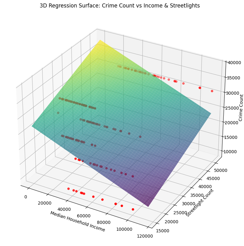
Regression: estimating relationships (OLS)
Finally,we ran OLS models to quantify relationships between income, streetlight count, and crime count:
- Model 1:
Crime_Count ~ MEDHINC_CY - Model 2:
Crime_Count ~ MEDHINC_CY + Streetlight_Count
# Model 1: Crime_Count ~ MEDHINC_CY
X_vt = sm.add_constant(merged_df["MEDHINC_CY"])
y_vt = merged_df["Crime_Count"]
model = sm.OLS(y_vt, X_vt).fit()

print("Model 1: Crime_Count ~ MEDHINC_CY")
print(model.summary())

# Model 2: Crime_Count ~ MEDHINC_CY + Streetlight_Count
X_light = sm.add_constant(merged_df[["Streetlight_Count", "MEDHINC_CY"]])
y_light = merged_df["Crime_Count"]
light_model = sm.OLS(y_light, X_light).fit()

print("\nModel 2: Crime_Count ~ MEDHINC_CY + Streetlight_Count")
print(light_model.summary())
Takeaways
- The analysis supports an inverse relationship between income and crime count at the ward level.
- Including streetlight count improves explanatory power and appears to matter alongside income.
- Classification models (RF/LR) provide a practical way to label wards as "high crime" based on a small set of features.
Next steps
- Make the pipeline fully reproducible outside Colab (local paths + env file)
- Add a dedicated evaluation for night crime prediction using
Night_Crime_Prop. - Consider stronger spatial methods (spatial lag/error models) for geographic dependence.