Urban Crime Data Analysis
Preface⌗
This blog post covers my part in a group data analysis project. If you would like the formal report detailing the process, findings, and conclusions complete with images and references you can find that here. Additionally, The official project showcase for this blog post can be found at in the Projects page.
What Was the Project About?⌗
Our goal was to understand how factors like neighborhood income and streetlight presence relate to crime rates in Tucson. We had two main questions:
-
Do thefts and violent crimes happen more in richer or poorer neighborhoods?
-
Does having more streetlights affect crime rates, especially at night?
To answer these, we used datasets from the City of Tucson, including police-reported crimes, arrest records, streetlight locations, and neighborhood income data. My role involved cleaning and merging these datasets, building visualizations, and helping with statistical models to test our hypotheses.
Data Cleaning and Prep⌗
The datasets were messy, with missing values and inconsistent formats. I used Python libraries like pandas and geopandas to:
-
Convert dates and times into a usable format (e.g., extracting hours from crime times to categorize them as Morning, Afternoon, Evening, or Night).
-
Standardize ward numbers across datasets for accurate merging.
-
Filter out irrelevant data, like inactive streetlights or missing coordinates.
-
Merge datasets by ward to create a unified dataset with crime counts, income levels, and streetlight counts.
This taught me how to handle real-world data, which is rarely perfect, and how to use tools like geopandas for spatial joins to connect streetlight locations with crime data.
Exploratory Data Analysis⌗
I created visualizations to spot patterns in the data:
-
A heatmap to show correlations between income, streetlights, crime counts, and nighttime crime proportions.
-
A scatter plot to visualize how crime counts relate to median income, with streetlight counts and nighttime crime proportions as additional dimensions.
-
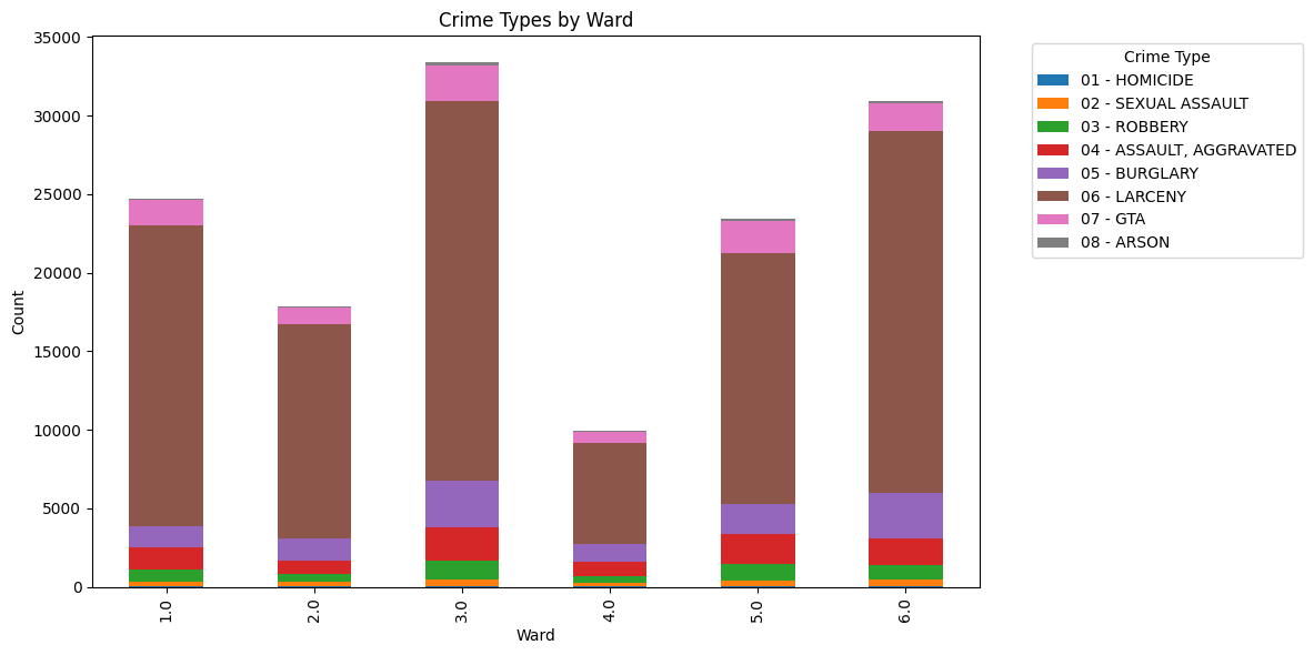
Stacked bar charts to show crime types (like larceny or robbery) across wards and time periods.
-
A histogram to track crime frequency by hour.
These visuals helped us see that larceny was the most common crime, especially in the afternoon, and that violent crimes like robbery spiked slightly at night.
Modeling and Analysis⌗
We used statistical and machine learning models to dig deeper:
-
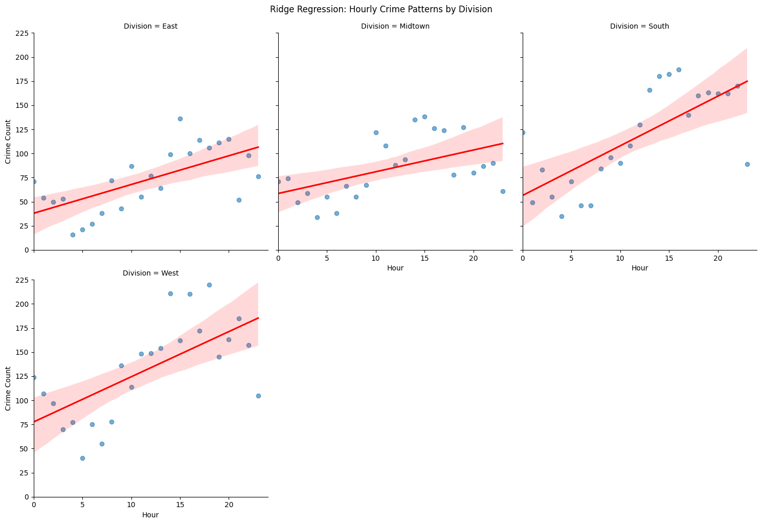
Ridge Regression: I helped analyze how crime counts varied by hour across Tucson’s police divisions (East, West, South, Midtown). This showed crime generally increases throughout the day, with South Division having the strongest trend.
-
Random Forest and Logistic Regression: We predicted whether a ward had high crime based on income and streetlight counts. I worked on scaling the data and evaluating model performance using metrics like accuracy and F1-score. The Random Forest model performed better, with 97% accuracy!
-
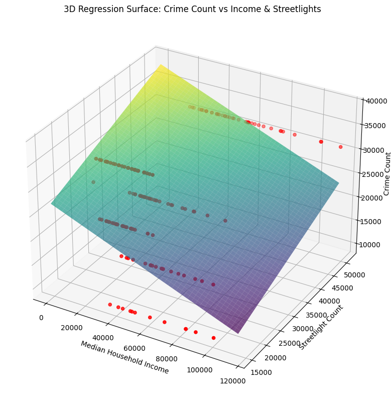
OLS Regression: We tested how income and streetlights predict crime counts. I contributed to interpreting the results, which showed that lower-income areas had higher crime rates, but more streetlights were linked to higher crime (likely because they’re placed in high-crime areas).
Key Findings⌗
-
Crime and Income: Lower-income neighborhoods, especially in Wards 3 and 5, had higher crime rates, supporting our first hypothesis. The OLS regression showed a significant negative relationship between median income and crime counts.
-
Streetlights and Crime: Surprisingly, areas with more streetlights had higher crime rates, which didn’t support our second hypothesis. This suggests streetlights are often installed in response to high crime rather than preventing it.
-
Crime Patterns: Larceny was the top crime across all wards, peaking in the afternoon. Violent crimes were more common at night but less frequent overall.
What I Learned⌗
This project was a huge learning experience for me:
-
Technical Skills: I got hands-on with Python libraries like pandas, seaborn, matplotlib, scikit-learn, and statsmodels. I also learned to work with geospatial data using geopandas.
-
Problem-Solving: Cleaning messy data and merging datasets taught me how to think critically about data quality and structure.
-
Teamwork: Collaborating with my teammates helped me improve my communication and project management skills.
-
Ethical Considerations: We discussed how our analysis could be misinterpreted (e.g., reinforcing stereotypes about low-income areas). This made me more aware of the ethical side of data science.